Let's illustrate a few simple calculations so you can see how DT works in the calculation process.
Consider the following simple model.
In this model, Cash is initialized at $0, and income is set at a constant of $100/month.
The following table shows the numerical values generated by the model. In the first run, DT is set to its default value of 0.25. In the second run, DT is set to 1.0. In each case, numerical values are printed every DT, stocks are reported as beginning balances, flows are reported as summed, and the "from" value for the simulation length is set to 0. Three months' worth of data appear in the tables.
In both runs, by Month 3, Cash totals $300. The only difference is the path followed in the two runs. In one case, $25 was added 12 times. In the other, $100 was added 3 times. In the first run, DT simply breaks the constant monthly flow of income into four equal chunks. Why would anyone want to do this?
As you'll soon see, there are a number of good reasons for breaking a time unit's worth of flow volume into smaller chunks. For now, a good first reason is that the division makes it possible to capture changes that occur over an interval of time less than the time unit you've picked for your model. When we picked a DT of 0.25, we would've been able to capture changes that occurred over an interval as short as 1/4 of a month (or roughly one week). So, DT represents the smallest time interval over which a change can occur.
DT thus determines how "chunkily" change will unfold in your model. A larger DT means chunkier changes in variables within your model. A smaller DT means smoother, more continuous changes.
Imagine creating a cartoon animation by riffling through a deck of static pictures. If you have a large deck of pictures, in which the change is small from one picture to the next, the animation will unfold smoothly as you riffle through the deck. By contrast, if you have a deck with only a few pictures, in which each picture represents a fairly big change relative to its predecessor, riffling through the deck will produce a jerky animation. DT works the same way with the numerical values in your model.
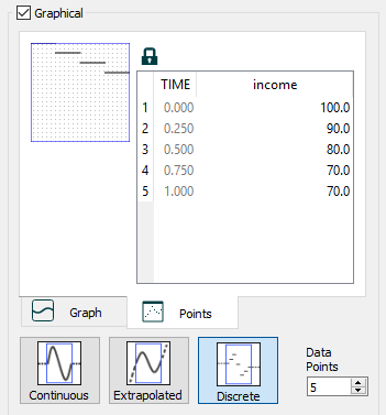
To illustrate the notion of change occurring within a unit of time, let's modify the Cash model to allow income to vary over a month. To implement variation, we'll convert income to a graphical function (using the discontinuous line segment option). The graphical function is shown below. The input to the graphical function is Months (running from 0 to 1.0, in increments of 0.25). The output of the graphical function is income, which now declines over the month.
We'll make two runs of the modified model. In the first, DT will be set to 0.25. In the second, we'll set DT to 1.0. Both runs will be one month in duration. Before looking at the results, do you think the value of Cash will be the same at the end of the two runs? If not, which run do you think will give a higher value of Cash?
The results from the two runs are presented below.
With DT set at 0.25, the value of income varies from DT to DT. Four calculations are made, each yielding a different value for income (each value is simply the value of income taken from the graphical function, and then multiplied by DT). Cash climbs to $85 by the end of the run. With DT set at 1.0, only one calculation is made. And so, only one value for income can be used. Given the way the graphical function works, that value is the value during Month 0. Cash grows to $100.
In summary, values of DT less than 1.0 enable your model to capture changes that occur within the course of a time unit. By adjusting DT, you can cause the changes in the variables in your model to unfold quite jerkily or very smoothly. The trade-off, for the most part, is speed against smoothness and numerical precision. As DT gets smaller, changes get smoother and results become more precise numerically; however, as DT gets smaller, more calculations will need to be made, and it will take longer to complete a run. As DT gets larger, results will be choppier and less precise numerically. But, a larger DT leads to fewer calculations and a faster simulation speed.