Imagine that you and three of your colleagues have been asked to run an obstacle course. You start at 1:00 PM, and complete the course at 1:35 PM. One of your colleagues starts at 1:05 PM, and completes the course at 1:42 PM. Your second colleague starts at 1:10 PM, and, being somewhat more athletic than you, completes the course at 1:35 PM. The third starts at 1:15 PM, gets stuck somewhere, and finishes at 2:15 PM. Because you know the start and end times for each person in the group, you can calculate a lot of useful information about the time that individuals (or groups of individuals) have spent "in process".
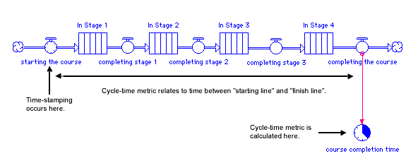
This little obstacle course example can be represented nicely as a stock/flow map. This next figure, for example, maps a four-stage course. As the figure suggests, incorporating cycle-time metrics into a model is very easy.
You'll note two distinctive features in this map. First, the flow "starting the course" looks a little like the face of a clock. The clock face on the flow indicates that the flow has been time-stamped. Whenever material moves through this flow, it'll be stamped with the current simulation time. Time-stamping establishes a starting time, so you can generate cycle-time metrics.
Second, the downstream flow "completing the course" has been connected to the converter called "course completion time". This converter also shows the face of a clock - but the face is partially filled. This partially-filled clock face indicates that the converter contains a cycle-time builtin function. When material moves through the downstream flow, the builtin will use the material's starting time information, in conjunction with the current simulation time, to calculate a cycle-time metric.