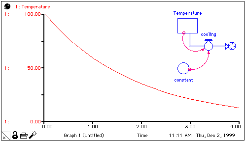
Consider the plot and model structure shown below.

The plot shows the idealized behavior of a real-world system; in this case, the temperature of a cooling cup of coffee. The model is idealized as well; if it were solved analytically, it would yield exactly the behavior exhibited by the plot.
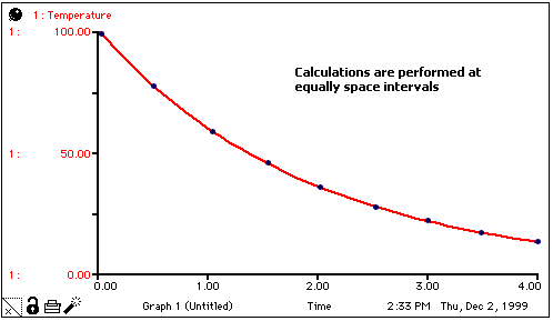
When the computer is used to simulate systems such as this, it's not possible to get an exact solution. Instead, a set of discrete calculations (the only kind that digital computers are capable of producing) is used to approximate the idealized curve. The software divides the time axis into equally-spaced intervals, each with a width of DT (or "delta time"). In this case, calculations are performed at discrete intervals, as indicated in the following graph.

In Stella, the equation structure that underlies the model diagram is of vital importance. The equations created behind the scenes as you hook together stocks and flows are known as "Finite Difference Equations." For example, on the Equation layer for the cooling model, there would be a set of equations that look like these:
Temperature(t) = Temperature(t-dt) + (-Cooling)*dt
INIT Temperature = 100
Cooling = Temperature * Constant
Constant = 0.5
In a model, each stock equation (in this case, the equation for Temperature) is a finite difference equation. Conceptually, solving finite difference equations is straightforward. It involves a two step initialization phase, and a three step iterative evaluation phase:
Step 1. Create a list of all stocks, and any flows or converters required to initialize those stocks, in the order of evaluation based on their equation. If a flow or converter has an initial equation that equation is used to determine the evaluation order.
Step 2. Calculate initial values for all stocks. Any flows or converters required to do this will also be computed (using their initial equations if they have them).
Step 3. Create a list of all flows and converters in the order of evaluation using their active equations.
Step 4. Calculate the values of all flows and converters based on the initial values of the stocks.
Step 1. Estimate the change in stocks over the interval DT. Calculate new values for stocks based on this estimate.
Step 2. Use new values of stocks to calculate new values for flows and converters.
Step 3. Update simulation time by an increment of DT. Stop iterating when Time >= simulation To Time.
Step 1 of the iteration phase is a critical one: How does one estimate the change in the value of stocks over the interval DT? The software provides diufferent algorithms for doing this estimation: Euler's method, 2nd-order Runge-Kutta, and 4th-order Runge-Kutta method.
You select the method your model will use in the Model Settings Properties panel box.