The statistical builtins perform a variety of statistical functions, or generate sequences of random numbers that conform to a specific distribution. The statistical builtins enable you to introduce randomness into your models. Random numbers are generated using a robust 64 bit generator, except as noted for RANDOM.
The builtins generating random number all take 4 optionalarguments (except RANDOM which only takes <seed>) .
Values are sample from the distribution you've specified, each DT during the model simulation. If you specify a value for seed other than NAN, the same values will occur every time the model is run. If you leave <seed> blank, or set it to NAN, then every time the model is run a different set of values will occur (it will not be possible to replicate the run).
Specifies the minimum acceptable value for the generated random number. This is useful when you want to truncate a distribution. Some distributions, such as NORMAL, can take on any values while other, such as POISSON, can only be positive integers. Setting a min is most useful for cases where some possible values are not reasonable. Leave empty or use NAN to specify no minimum.
Specifies the maximum acceptable value for the generated random number. This is useful when you want to truncate a distribution. Some distributions, such as NORMAL, can take on any values while other, such as POISSON, can only be positive integers. Setting a max is most useful for cases where some possible values are not reasonable. Leave empty or use NAN to specify no minimum.
Specified how frequently values will change. Normally generated values change every DT, but you can specify a larger number if you want to have them stay constant over an interval. For example, using 1 will keep the same during each unit time interval changing only at time 1, 2, 3 and so on independent of DT.
Note For some distributions, such as uniform, it really does not make sense to specify another minimum and maximum, however, the argument sequence is kept for consistency so to specify a sample time you will need to include the min and max (using NAN for each is easiest).
This section describes the following builtins:
The BETA builtin generates a series of random numbers that conforms to a beta distribution defined by two shape parameters, alpha and beta. The BETA builtin samples from continuous distributions.
The BINOMIAL builtin generates a series of random numbers from a discrete probability distribution of the number of successes in a sequence of trials with a given success probability. The success probability should be a number between 0 and 1 (numbers outside the range are set to 1).
The negative binomial builtin is a discrete number generator that will only return integers, and treats the number of trials as an integer (similar to MONTECARLO, NEGBINOMIAL, and POISSON).
The COMBINATIONS builtin calculates the number of r-element subsets (or r-combinations) of an n-element set. The mathematical notation for this calculation is: n! /[r! * (n-r)!]
Example:
COMBINATIONS(5, 3) = (5 * 4 * 3 * 2 * 1) /[(3*2*1)*(2*1)] = 10
The EXPRND builtin generates a series of exponentially distributed random numbers with a mean of lambda. EXPRND samples a new random number in each iteration (that is, each DT) of a model run. If you want to replicate the stream of random numbers, specify seed as an integer between 1 and 32767. To replicate a simulation, all variables that use statistical functions must have seeds specified. Each variable using a statistical function should use a separate seed value.
Examples:
EXPRND (1) gives a non-replicable exponentially distributed stream of numbers (mean=1)
EXPRND (2,1456) gives a replicable exponentially distributed stream of numbers (mean=2)
The FACTORIAL function calculates the factorial of n (traditionally noted as n!).
Example:
FACTORIAL(5) = 5 * 4 * 3 * 2 * 1 = 120
The GAMMA builtin generates a series of random numbers that conforms to a gamma distribution with the specified shape and scale. If unspecified, scale uses the value 1.0. The GAMMA function samples from continuous distributions.
The GAMMALN builtin returns the natural log of the GAMMA function, given input n. The GAMMA function is a continuous version of the FACTORIAL builtin, with GAMMA(n) the same as FACTORIAL(n-1). Because this builtin returns the log of the result, it's possible to call it with larger arguments than FACTORIAL. This makes it very useful for computing ratios of different factorials. For example, EXP(GAMMALN(1001) - GAMMALN(951) - GAMMALN(51)) is the same as COMBINATIONS(1000,50).
The GEOMETRIC builtin generates a series of random numbers from a discrete probability distribution of the number of trials before the first success with a given success probability. The success probability should be a number between 0 and 1 (numbers outside the range are set to 1).
The GEOMETRIC builtin samples from discrete distributions (as the MONTECARLO and POISSON functions do).
The INVNORM builtin calculates the inverse of the NORMALCDF builtin .
The LOGISTIC builtin generates a series of random numbers that conforms to a logistic distribution with a specified mean and scale. The LOGISTIC builtin samples from continuous distributions.
The LOGNORMAL builtin generates a series of random numbers that conform to a Log-Normal distribution (that is, the log of the independent variable follows a normal distribution) with a specified mean and stddev (standard deviation). LOGNORMAL samples a new random number in each iteration of a simulation. If you want to replicate the stream of random numbers, specify seed as a positive integer. To replicate a simulation, all variables that use statistical functions must have seeds specified. Each variable using a statistical function should use a separate seed value.
Examples:
LOGNORMAL(0,1) gives a non-replicable stream of numbers following a log-normal distribution (mean=0, standard deviation=1)
LOGNORMAL(0,1,147) gives a replicable stream of numbers following a log-normal distribution (mean=0, standard deviation=1)
LOGNORMAL(5,1,12) gives a replicable stream of numbers following a log-normal distribution (mean=5, standard deviation=1)
LOGNORMAL(10,5,102) gives a replicable stream of numbers following a log-normal distribution (mean=10, standard deviation=5)
The MONTECARLO builtin randomly generates a series of zeros and ones from a Bernoulli distribution based on the probability you've provided. The probability is the percentage probability of an event happening per DT divided by DT (it is similar too, but not the same as, the percent probability of an event per unit time). The probability value can be either a variable or a constant, but should evaluate to a number between 0 and 100/DT (numbers outside the range will be set to 0 or 100/DT). The expected value of the stream of numbers generated summed over a unit time is equation to probability/100.
MONTECARLO is equivalent to the following logic:
IF (UNIFORM(0,100,<seed>) < probability*DT THEN 1 ELSE 0
MONTECARLO samples a new random number in each iteration of a model. If you want to replicate the stream of random numbers, specify seed as a positive integer. To replicate a simulation, all variables that use statistical functions must have seeds specified. Each variable using a statistical function should use a separate seed value.
Examples:
MONTECARLO(20,1577) with a DT of 1 gives a replicable stream of numbers, which are equal to 1 20% of the time and equal to 0 the remaining 80% of the time.
The MONTECARLO builtin samples from discrete distributions (as BINOMIAL, NEGBINOMIAL, and POISSON do).
The NEGBINOMIAL (Negative Binomial) builtin generates a series of random numbers from a discrete probability distribution of the number of failures in a sequence of trials with a given success probability that result in the specified number of successes. The success probability should be a number between 0 and 1 (numbers outside the range are set to 0 or 1).
The negative binomial builtin is a discrete number generator that will only return integers, and treats the number of successes as an integer.
The NORMAL builtin generates a series of normally distributed random numbers with a specified mean and stddev (standard deviation). NORMAL samples a new random number in each iteration of a simulation. If you want to replicate the stream of random numbers, specify seed as a positive integer. To replicate a simulation, all variables that use statistical functions must have seeds specified. Each variable using a statistical function should use a separate seed value.
Examples:
NORMAL(0,1) gives a non-replicable normally distributed stream of numbers (mean=0, standard deviation=1)
NORMAL(0,1,147) gives a replicable normally distributed stream of numbers (mean=0, standard deviation=1)
NORMAL(5,1,12) gives a replicable normally distributed stream of numbers
(mean=5, standard deviation=1)NORMAL(10,5,102) gives a replicable normally distributed stream of numbers (mean=10, standard deviation=5)
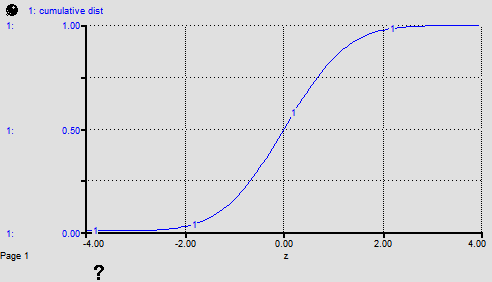
The NORMALCDF builtin calculates the cumulative Normal distribution function between the specified z-scores, or, when the mean and stddev (standard deviation) are given, between two data values. The cumulative distribution function integrates (sums) all values of the Normal probability distribution function between the left and right endpoints. To sum from negative infinity, use a z-score of -99. To sum to positive infinity, use a z-score of 99.
The following graph shows the behavior of the NORMALCDF function for -4 = z = 4.
The equation NORMALCDF(-99, TIME) was used to make this graph. Note that the NORMALCDF very closely approximates the logistic function, or S-shaped growth. It can be used to formulate, using an equation, several types of common graphical functions:
Note: A z-score can be calculated with the formula: (data_value - mean)/stddev.
The PARETO builtin generates a series of random numbers that conforms to a distribution whose log is exponentially distributed with a specified shape and scale. The PARETO builtin samples from continuous distributions.
The PERMUTATIONS builtin calculates the number of permutations of an n-element set with r-element subsets. The mathematical notation for this calculation is: n!/(n-r)!
Example:
PERMUTATIONS(5,3)=5*4*3*2*1/2*1=60
The POISSON builtin generates a series of random numbers that conform to a Poisson distribution. The mean value of the output is mu * DT, and the output should be used with the PULSE function when computing flows. For example, the inflow PULSE(POISSON(3.5)) will have an average value of 3.5 (per time unit) and will always cause the level to change by an integer value. POISSON samples a new random number in each iteration of a model run (that is, every DT). If you want to replicate the stream of random numbers, specify seed as an integer between 1 and 32767. To replicate a simulation, all variables that use statistical functions must have seeds specified. Each variable using a statistical function should use a separate seed value.
Examples:
POISSON (1) gives a non-replicable Poisson sample set with mean of 1*DT.
POISSON (10,1256) gives a replicable Poisson sample set with mean of 10*DT.
The POISSON builtin returns the units of measure as mu multiplied by the units for time. You can specify a flow rate and then, when used with the PULSE function as described above, the units will be correct.
The POISSON builtin always returns an integer.
The RANDOM builtin is the same as the UNIFORM builtin, except that it uses the older version of the random number generator used in the version of iThink/STELLA before version 10.1. It's kept to support models that depended on its behavior. Specify seed as an integer between 1 and 32767.
The TRIANGULAR builtin generates a series of random numbers that conforms to a triangular distribution with a specified lower bound, mode, and upper bound. The TRIANGULAR builtin samples from continuous distributions.
The UNIFORM builtin generates a series of uniformly distributed random numbers between min and max. UNIFORM samples a new random number in each iteration of a model run. If you want to replicate the stream of random numbers, specify seed as positive integer. To replicate a simulation, all variables that use statistical functions must have seeds specified. Each variable using a statistical function should use a separate seed value.
Examples:
RANDOM(0,1) creates a non-replicable uniformly distributed stream of numbers between 0 and 1.
RANDOM(0,1,147) creates a replicable uniformly distributed stream of numbers between 0 and 1.
RANDOM(0,10,12) gives a replicable uniformly distributed stream of numbers between 0 and 10.
RANDOM(10,13,12) gives a replicable uniformly distributed stream of numbers between 10 and 13.
The WEIBULL builtin generates a series of random numbers that conforms to a Weibull distribution with the specified shape and scale. The WEIBULL builtin samples from continuous distributions.