 stock = dt * flow
By far the simplest algorithm used by the software is Euler's method. In this method, the computed values for flows provide the estimate for the change in corresponding stocks over the interval DT. In the simple cooling model, the initialization and iteration phases look like this:
Step 1. Create a list of all stocks, flows, and converters, in required order of evaluation.
Step 2. Calculate initial values of all stocks, flows, and converters (in order of evaluation).
Time = From Time
--->Time = 0
Stockt=0 = f(initial values, stocks, converters, flows)
--->INIT Temperature = 100
Converters = f(stocks, converters, flows)
--->constant = 0.5
Flows = f(stocks, converters, flows)
--->cooling = Temperature * constant
Step 1. Estimate change in stocks over the interval DT.
Calculate new values for Stocks based on this estimate.
Stockt = Stockt-dt +
--->Temperature = Temperature + (-cooling) * dt
Step 2. Calculate new values for flows and converters (in order of evaluation).
Converters = f(stocks, converters, flows)
--->constant = 0.5
Flows = f(stocks, converters, flows)
--->cooling = Temperature * constant
Step 3. Update simulation time. Stop iteration when Time >= simulation stoptime.
Time = Time + dt
The numeric output generated by the cooling model, for the first four time units, is shown in the following table. The output was produced using Euler's method, with DT = 0.5, beginning balances, and summed reporting of flows.
As the above data show, cooling declines in proportion to Temperature. The data set for Temperature approximates an exponential decay pattern, such as the one shown in How model equations are solved.
At this point, however, it's useful to ask about the accuracy of this approximation. As the following graph shows, the model output is not very accurate when compared with the analytical solution to the equivalent equation (Temperature = 100e-0.5*time). Because Euler's method simply uses the value calculated for the flow as its estimate for the change in the stock over the interval DT, and because the interval is a large one (relative to the continuous case), an integration error is introduced. This integration error is the difference between the two curves on the plot.
When you select Cycle-time as the integration method, the software uses Euler integration, so the computation proceeds exactly as described above. What changes is the information recorded. When cycle-time is selected, non-negative Stocks are changed to track their inflow and outflow information the same way that Queues do. For example, consider a simple processing model:
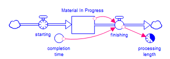
In this model the computation would occur the same way it was described above. During the integration step, however, instead of simply adding starting to, and subtracting finishing from, Material in Progress, actions are taken in sequence. First, starting is added and marked as the most recently added material. Then, finishing is used to remove material, beginning with the least recently added material and continuing to more recently added material as necessary. In this example, finishing will never reach the material just added by starting, but in other cases, it might. The single Stock Material in Progress, instead of being just a single quantity, is broken up into a sequence of values, arranged by the length of time they've been inside the stock. As material exits, the software knows how long it's been in the Stock; this information is used to compute processing length.
Thus, with cycle-time active, the behavior at the macro level is the same, but additional information is retained in order to report the cycle-time metrics.